Sensitivity Analysis with SALib

Sensitivity analysis is the "study of how the uncertainty in the output of a mathematical model or system can be apportioned to different sources of uncertainty in its inputs" [Wikipedia].  Sensitivity analysis is a powerful technique for gaining insight into a model by understanding in general terms how the model's output is influenced by the model's inputs.  In this post, we provide a short introduction to sensitivity analysis using visual scatter plots followed by an introduction of SALib, an open source Python library for sensitivity analysis.

SA using Scatter Plots

Sensitivity analysis can be demonstrated visually using scatter plots.  Suppose we have a model, y = f(x) + ε, with a single input, x, and an error term, ε.  We can generate a scatter plot by randomly sampling values of x and recording the output y:

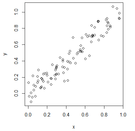
In this example, we observe that increasing values of x result in increasing values of y.  This indicates there is a positive correlation between x and y, which is implies that changing the value of x has a direct influence on the value of y.  If we fit a line to these points, the sensitivity is the slope of the line.  In this example, the sensitivity is approximately 1.  Any increase or decrease in the value of x results in a proportional change to y.

Take for example the following:

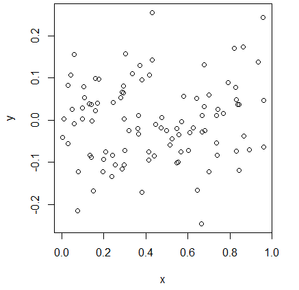
In this case, the slope of the line is 0, indicating the sensitivity of y given x is 0.  The value of y is independent of the value of x.

Suppose now we have a function with two inputs, y = f(x1, x2) + ε.  Like before, we sample x1 and x2 independently and generate the scatter plot.  The black points show the output caused by varying x1 and the red points show the output caused by varying x2.

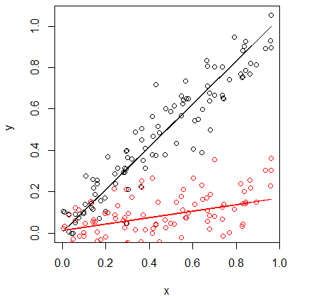
The steeper slope of the black line with respect to the red line indicates that y is more sensitive to x1 than x2.  Furthermore, the relative slope of the lines indicates the relative magnitude of the sensitivities.  In this example, y is approximately 5 times more sensitive to changes in x1 than x2 (since the slope of the black line is ~1.0 and the slope of the red line is ~0.2).

Using SALib

This visual approach is useful for simple models, but can be challenging to use and error prone for more complex models.  To address these issues, a variety of sensitivity analysis methods have been developed over the years.  These methods typically calculate what are called sensitivity indices as numeric values.  Depending on the specific method, they can compute:

1. First-order indices: measures the contribution to the output variance by a single model input alone.
2. Second-order indices: measures the contribution to the output variance caused by the interaction of two model inputs.
3. Total-order index: measures the contribution to the output variance caused by a model input, including both its first-order effects (the input varying alone) and all higher-order interactions.

SALib is an open source library written in Python that contains a variety of sensitivity analysis methods.  To download and install SALib, we you will first need to install Git and Python.  Next, run the following commands.

    git clone https://github.com/SALib/SALib.git
    cd SALib
    python setup.py develop

To demonstrate the use of SALib, we will perform a Sobol’ sensitivity analysis of the Ishigami function, shown below. The Ishigami function is commonly used to test uncertainty and sensitivity analysis methods because it exhibits strong nonlinearity and nonmonotonicity.

To begin, start a new interactive Python session.  Next, import the necessary libraries. In SALib, the sample and analyze functions are stored in separate Python modules. For example, below we import the saltelli sample function and the sobol analyze function. We also import the Ishigami function, which is provided as a test function within SALib. Lastly, we import numpy, as it is used by SALib to store the model inputs and outputs in a matrix.

Importing Python Libraries

​Next, we must define the model inputs. The Ishigami function has three inputs, x1, x2, and x3, where x ∈ [-π, π]. In SALib, we use a dict defining the number of inputs, the names of the inputs, and the bounds on each input, as shown below.

Defining Problem

Next, we generate the samples. Since we are performing a Sobol’ sensitivity analysis, we need to generate samples using the Saltelli sampler, as shown below.

Generating Input Samples

Here, param_values is a NumPy matrix. If we run param_values.shape, we see that the matrix is 8000 by 3. The Saltelli sampler generated 8000 samples. The Saltelli sampler generates N*(2D+2) samples, where in this example N is 1000 (the argument we supplied) and D is 3 (the number of model inputs).

Next, we must evaluate the model using our generated samples.  In this example, we are using the Ishigami function provided by SALib. We can evaluate these test functions as shown below:

Evaluating the Model

With the model outputs computed, we can finally compute the sensitivity indices. In this example, we use sobol.analyze, which will compute first, second, and total-order indices.

Analyze the Outputs

Si is a Python dict with the keys "S1", "S2", "ST", "S1_conf", "S2_conf", and "ST_conf". The _conf keys store the corresponding confidence intervals, typically with a confidence level of 95%. We can print the values as shown below.

>>> # Print the first-order indices
>>> print Si['S1']
[ 0.30644324  0.44776661 -0.00104936 ]

>>> # Print the total-order indices
>>> print Si['ST']
[ 0.56013728  0.4387225   0.24284474]

>>> # Print the interactive effects
>>> print "x1-x2:", Si['S2'][0,1]
>>> print "x1-x3:", Si['S2'][0,2]
>>> print "x2-x3:", Si['S2'][1,2]
x1-x2: 0.0155279
x1-x3: 0.25484902
x2-x3: -0.00995392

From this output, we make several observations.  First, x1 and x2 show strong first-order sensitivities, but x3 has no first-order sensitivity.  x3 has interactive effects as seen by the second and total-order indices.

Conclusion

SALib is a powerful toolbox for sensitivity analysis.  In this post, we walked through an example using Sobol' sensitivity analysis.  SALib includes other methods, including the Fourier Amplitude Sensitivity Test (FAST), Method of Morris, and Delta-Moment Independent Measure.

We also want to note that while SALib is a Python library, it is designed to work with models in any form.  SALib includes a convenient command line interface for generating the model inputs and analyzing the model outputs.  Additional documentation for SALib is available online at ReadTheDocs.